Make a chart
c charts the rows left after the query and filters. It starts with a chart that suits the column under the column cursor. Esc returns to the table.
| Cursor column | Chart c opens |
|---|---|
| A number | Its histogram |
| Text, categorical or boolean | A bar of its counts per value |
| A date or a time | A line of the first numeric column over it (with no numeric column, Y is left for you to pick) |
Until you change the type, the panel says suggested for f64 under Type.
Pressing c again on the same column of the same dataset brings back
the chart as you left it. On another column, it suggests a new chart.
The panel
The panel on the left holds four shelves, the same four for every type,
followed by the options. A shelf the chart type does not use stays in place,
dimmed, with the reason beside it (density, same as X). Moving through the
panel skips it.
| Shelf | Holds | Under it |
|---|---|---|
| Type | Line, Scatter, Bar, Histogram, Box, KDE, Heatmap | suggested for <type> |
| X | The column on the X axis | The time bucket of a date X on a line or scatter; the bar order; the histogram’s bins |
| Y | A column, or several on a line or scatter (one series each); on a histogram, count or share | On a line, scatter or bar, the Aggregate row, and cumulative when it is on |
| Color | Category, date or datetime columns: one series per value, or per combination of several columns’ values | Which values: top 10 of 16 by rows, all 3, 3 picked of 4,812 |
The plot’s title row says how the rows were combined: mean by month, running sum, colored by carrier, count per bin, one box per carrier.
Column names go on the axes instead: Y above the y axis, X below the right end
of the x axis. So a plain line or scatter has a blank title row. At the right
end of the title row, dimmed, the chart says which rows it read: sample of 10,000 of 337k rows · seed 42891, 1,207 values outside p1-p99. The seed
draws the same sample again; a chart of every row shows no seed. When the row
is too narrow for both, these notes are cut short with … or left out.
Plot two columns
Open Palmer penguins from Example datasets, as in the quick start, then:
- Press c, then 2 for Scatter.
- Choose
flipper_length_mmfor X andbody_mass_gfor Y.
Use ↓ to move through the panel’s rows and Space to open a shelf’s picker. Type part of a name to narrow the list. On Y, Space toggles a column and Enter closes the picker, which leaves out the X column. The chart leaves out the two penguins with no measurements.
Points are drawn in X order, so a line runs left to right whatever order the table is in. Nulls are dropped per series: a row with no X is left out, and a missing Y drops that series’ point and breaks its line. Other series keep their points.
Esc keeps the chart as you left it. Sort or filter the table, press c on the same column, and the same shelves chart the new view. A column the view no longer has is dropped from the chart. Opening another dataset starts over.
Aggregate
On a line, scatter or bar chart, the Aggregate row under Y combines
rows. ← → step through none, count, distinct, sum, mean,
median, stdev, quantile, min, max, first and last. With an aggregate, the rows
that share an X (and a color) become one point or one bar. It runs over every
row of the view, as one group-by in the background, and the footer shows
Grouping 337k rows... meanwhile. The title row says how many rows it used:
all 336,776 rows, or rows in the groups shown when Color leaves values out
and Other is off. Without an aggregate, a chart samples, and says so.
| Aggregate | Each point or bar | Y |
|---|---|---|
| count | The rows | None needed |
| distinct | The different values, nulls left out (nunique in a query counts a null as one) | Any column, text too. Switching to another aggregate drops a text Y |
| sum, mean, median, min, max | As named | A number |
| stdev | The sample standard deviation (n − 1). A group of one row has none and draws no point | A number |
| quantile | The percentile on the line under Aggregate, p90 to start; ← → there step 1, 5, 10, 25, 75, 90, 95 and 99. Linear interpolation between the two nearest values | A number |
| first, last | The first or last non-null value in the view’s order: its sort, which Aggregate names (last · by time_hour ▲), or else the order the rows were read in (last · by row order) | A number |
| Option | What it does |
|---|---|
| Time bucket | Line and Scatter, under a date or datetime X: none, day, week (from Monday), month, quarter, year. Picking a bucket with no aggregate sets mean; picking an aggregate on a date X with no bucket sets day |
| Cumulative | Line and Scatter, with count, sum, mean, median, min or max: off, running sum, or compound. The other aggregates have none, since a running sum of distinct counts, deviations, percentiles or first values is not that measure so far. The rows are totaled in X order, per series, and each point is the total at the end of its X or bucket: a running sum of Y, or Y’s rates compounded over every row, (1 + y1)(1 + y2)… − 1. While it is on, the aggregate is set aside (a count becomes a running count of rows) and Aggregate says so: mean · compound of rows |
If a sample of X shows more than about 200,000 different values, the chart is refused before any rows are grouped, with advice to bucket X by a time unit or choose an X with fewer values.
On NYC flights (2013), with no query: press c on carrier, pick
arr_delay for Y and step the aggregate to mean. Sixteen bars, F9
longest at 21.92 minutes; HA and AS arrive early on average, so their bars
grow left of zero.
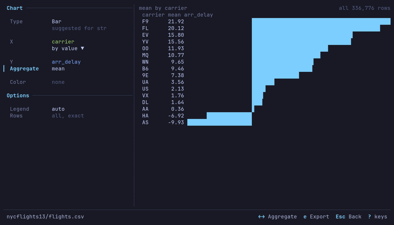
Which airlines arrive late? F9, by 21.92 minutes on average. c on
carrier, Y arr_delay, → on Aggregate to mean.
Color
Color splits a chart into one series per value of a category, date or datetime column, each in its own palette color. Until you pick values, the ten values with the most rows are drawn (or all of them, when the view has fewer), and the line under Color says which. Space on that line lists every value with its row count, most first. Type to narrow the list, Space toggles a value (up to ten), and Enter charts the ones picked. Values are counted over the whole view.
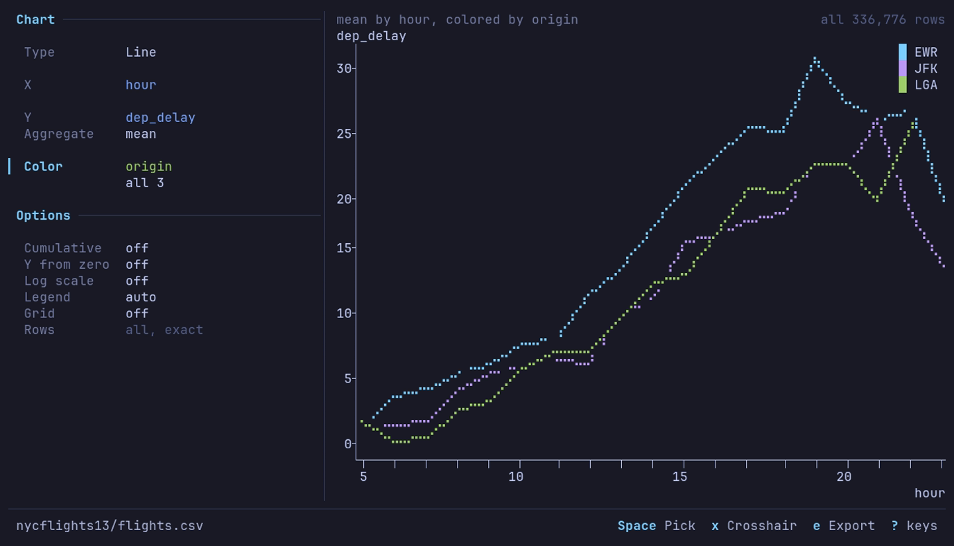
Which New York airport leaves latest, and when? Newark in the evening,
31.1 minutes on average at 19:00. A line of dep_delay by hour,
Aggregate mean, Color origin.
Other groups the values without a series of their own into one more
series, drawn in dimmed and listed last in the legend. ←
→ on the line under Color turn it on or off. The line then reads
top 10 + 6 other or 3 picked + 4,809 other. It starts on for a scatter and off for the other
types. When every value has a series there is no Other.
| Type | With Color |
|---|---|
| Line, Scatter | A line or set of points per value. Other is one more line, aggregated over the rest as the others are; on a scatter its points are drawn under the colored ones, so the cloud keeps its shape. Several Y columns are already one series each, so Color is dimmed |
| Bar | A bar per value in each category’s row, under a legend of the values; Other is one more bar per category. Needs an aggregate |
| Histogram | Each value’s bins drawn as an outline, since filled bars would hide each other. Y can be share of group: each bin’s share of its group’s rows inside the range, so groups of different sizes compare. Other is one more outline. The range (p1-p99) is taken from the whole column |
| KDE | A curve per value; Other is one more |
| Box | Dimmed: a category on X already makes one box per value, for the ten values with the most rows |
| Heatmap | Dimmed |
A null value is a series of its own, named null.
Several columns
Space on Color opens its picker, where Space toggles
columns in the order you pick them and Enter charts them. With none
toggled, Enter takes the column under the cursor alone. Each
combination of their values is one series, named by the values joined with ·:
FlightSimulator2024 · 2026-10-22 18:40:30. Counts, the top ten, the value
picker and Other work per combination. ← → on Color
step to a single column. none clears them.
Dates and datetimes are written as ISO 8601 with a space before the time:
| Column | Written |
|---|---|
| Date | 2026-10-22 |
| Datetime | To the minute, with seconds and a fraction only as far as some value needs them: 2026-10-22 18:40, 2026-10-22 18:40:30, 2026-10-22 18:40:30.250 |
| Datetime with a time zone | The zone’s abbreviation after it: 2026-10-22 14:40 EDT |
Chart types
| Type | Plots | X | Y |
|---|---|---|---|
| Line | Lines in X order | A number, date, time or duration | Up to ten number or duration columns, or a count |
| Scatter | Points | A number, date, time or duration | Up to ten number or duration columns, or a count |
| Bar | One horizontal bar per category | A text, categorical, boolean or integer column | A numeric column with an aggregate, a count, or a column already one row per category |
| Histogram | Rows per bin | A number | Count or share |
| Box | Quartiles and whiskers | A category, one box per value, or none | A number |
| KDE | A smoothed density curve | A number | Density |
| Heatmap | Density of two variables | A number | A number |
| Option | Types | What it does |
|---|---|---|
| Bins | Histogram (under X), Heatmap | 5 to 100 bins for a histogram, 5 to 60 a side for a heatmap |
| Bandwidth | KDE | A multiple of the usual bandwidth, 0.2x to 5.0x |
| Range | Histogram, Box, KDE, Line, Scatter | So outliers do not squash the rest. A histogram, box or KDE takes All values or p1-p99, the 1st to 99th percentile, and counts the values it left out: 1,207 values outside p1-p99. A line or scatter chart takes All or outliers at edge: it keeps every point, spans its Y axis over those that are not outliers (as Distribution counts them), and draws the outliers at the edge: 2 outliers at the edge. The crosshair reads their true values |
| Smooth | Line | Draw each point as the mean of the values in a window ending at it (a moving average), to show the trend through noisy readings: off, or a window, a length of time or a number of points. See Smoothing |
| raw (under Smooth) | Line | Draw the raw line faintly behind the smoothed one: auto (with one series), on or off |
| Trend | Scatter | A line fitted through the points: off, linear, exponential, power, robust, local or y = x. See Trend lines |
| over (under Trend) | Scatter | With a Color: one fit per color, or one over all points |
| Order | Bar (under X) | By value, largest first, or by label: text A to Z, numbers ascending |
| Y from zero | Line, Scatter | Start the Y axis at zero. Dimmed while Y is on a log scale, which has no zero |
| Log scale | Line, Scatter | Y, and X on the line under it: a log axis. See Log scale |
| Legend | Line, Scatter, Bar, Histogram, KDE | auto or off |
| Grid | Line, Scatter, Histogram, Box, KDE | Lines at the labeled ticks |
| Rows | Charts that sample | Sample of a size, or Every row; an aggregate reads every row and says all, exact. See Large tables |
Smoothing
Readings that jump around, such as frame times, sensor values or daily delays, can hide their trend. Smooth draws a moving average (trailing mean): each point is the mean of the values in a window that ends at it, so the trend shows through. The price is that a mean lags: a real change shows up late on the smoothed line, and a short spike is flattened. The lag is about half the window. A longer window gives a smoother line that lags more. The raw line, drawn faintly behind, keeps both in view.
Focus Smooth with Tab and step the window with ← →. Once a window is on, the row under it, raw, says whether the raw line is drawn.
| Setting | Values |
|---|---|
| Smooth | off, or a window. Over a date, datetime, time or duration X, a length of time: 7d, 1m (a minute). Over any other X, a number of points: 20 points |
| raw | auto draws the raw line when the chart has one series and leaves it out with several, where it would crowd the plot. on always, off never. Each raw line is its series’ color, faded |
What the screen says:
| Where | What |
|---|---|
| Title row, right | mean of the trailing 7d, with or without the raw line |
| Crosshair (x) | Each series’ smoothed value, then its raw value: delay: 21.255 (raw 83.536921). The smoothed value is rounded to one decimal more than the raw value, up to three, since a mean’s later digits are noise. A duration Y is written as usual |
| Panel | off · too few points when no window would average more than one point; off · steps too big when every step of an envelope holds more rows than the longest window; off · line only on a Scatter chart |
The windows offered fit the data: over time, those longer than the median gap between points and at most half the X span; over numbers, at most half the longest series, and on an envelope more rows than its biggest step holds. When fewer than three fit, up to three are offered, the shortest longer than that gap, none longer than the span.
How it is worked out
| Part | Rule |
|---|---|
| Mean | A trailing mean with no look-ahead. A point at X with a window of length w averages the values with X in (X − w, X], so points that share an X are all included. A window of N points averages the point and the N − 1 before it |
| Start of a series | The first points average only the points so far, so they are noisier |
| Nulls | Skipped. A window with no values draws no point (∅ at the crosshair) |
| Series | Each smoothed on its own, after any bucket, aggregate and cumulative |
| Large tables | A line drawn as an envelope (see Large tables) averages the rows behind each step, not its lowest and highest value, and a window of N points is N rows, the oldest step counted in part, at its mean: min and max of 192M rows in 5,000 steps · mean of the trailing 1m |
| Order | Smoothed, then (on a log scale) the points at 0 or less left out, then Range, then Log scale |
| Range | With outliers at edge: without the raw line, the Y axis spans the smoothed line less its outliers. With it, the axis spans both lines less their outliers, and each line’s outliers are drawn at the edge and counted in the title row. With All, the axis spans the raw line too; hide it (raw off) or use outliers at edge to fit the smoothed line |
Smoothing changes only the drawing, not the data. An export draws the smoothed line over the faded raw line as the screen does.
Example: a week’s mean of daily delays
Open NYC flights (2013) from Example datasets on the home screen, press : and run the mean departure delay of each day (as in Querying data):
SELECT DATE(CONCAT_WS('-', year, month, day)) AS flight_date,
       AVG(dep_delay) AS delay
FROM df
GROUP BY flight_date
ORDER BY flight_date
With the cursor on flight_date, press c: a line of delay per
day. Tab to Smooth and press →. Daily points over a
year offer 7d, 30d and 90d, and the first step is 7d. The title row
says mean of the trailing 7d, and the raw line stays behind the smoothed one,
as the chart has one series. Press x and move to 2013-03-08: the
readout says delay: 21.255 (raw 83.536921). That day stands out at 83.5
minutes, but its week’s mean is 21.3.
Log scale
Some values span many orders of magnitude: file sizes, city populations, response times. On an ordinary axis the largest few take the whole width and the rest crowd into a strip at zero. A log axis gives each power of ten the same room, so 1 to 10 is as wide as 1,000 to 10,000. Equal steps along it are equal ratios, not equal differences: doubling looks the same anywhere on the axis.
Log scale has two lines: Y on its own row and X on the line under
it. Focus either with Tab and toggle it with Space. X
takes only a number X: over a date, time or duration X the line reads
X numbers only, dimmed, and Tab skips it.
Both axes follow the same rules:
| Part | Rule |
|---|---|
| Values of 0 or less | A log has no place for them, so they are left out and counted in the title row: 3 points with Y ≤ 0 left out, or with X or Y when both axes are logged (<= in ASCII). A line breaks where they were. A series with none left is named there too: size: every point left out. With nothing left at all, the plot says so |
| Ticks | Powers of ten (1, 10, 100), with 2 and 5 between when there is room, or every second or third power when there is less. An axis spanning less than a power of ten ticks at round steps (200, 400, 600). The axis ends where the data does; one value alone gets half a power of ten each side |
| Labels | Each with the digits it needs: 0.01 1 100. Past four powers of ten, or a label longer than six characters, all in a short form: 1 1k 1M from one up, 1e-9 1e-3 1 1e3 below it. Round steps within a power of ten share one precision: 0.5 1.0 1.5 |
| Crosshair | Steps between the points drawn, skipping those left out, and reads the data’s own values: size: 100, not 2 |
| Smooth | A window averages every point, including those left out, so the smoothed line can run above 0 where the data is 0. Each line then draws only its own points above 0. The note counts the smoothed line’s: 4 smoothed points with Y ≤ 0 left out, and the raw line’s too when it is drawn |
| Range | Fits the Y axis to the points drawn, not those left out. On a log Y the outliers are found on the log scale, so a steady climb through powers of ten has none |
| Duration Y | Ticks named as lengths of time: 10ms, 1s, 1m40s |
| Y from zero | Dimmed while Y is logged |
| Large tables | A line drawn as an envelope (see Large tables) steps evenly along a log X, so each power of ten gets its share of the steps, and counts the rows left out: 12 rows with X ≤ 0 left out. Turning X on or off reads such a line again. On a log Y each step stands on its least value above 0, and the rows with Y of 0 or less are counted (values, with several Y columns): 9,355 rows with Y ≤ 0 left out. Turning Y on or off only redraws |
| Export | Draws the same axes and notes |
Before 0.4.14, Y drew ln(1 + y), which kept 0 on the axis. A saved view with Y on now draws log10 and leaves its zeros out.
Example: flight distances
Open NYC flights (2013) from Example datasets, press c, set
the type to Scatter, X to distance and Y to air_time. Distances run
from 17 to 4,983 miles, and more than half the flights are under 1,000, so on
an ordinary axis they crowd into the left fifth of the plot. Tab to X under
Log scale and press Space: those flights now spread over more
than half the width, and the short hops under 200 miles separate.
Trend lines
A scatter shows how two columns move together; a trend line says how much.
Trend fits a line through the points, draws it over them in its own color
(the theme’s chart_trend; the points fade behind it) and reads it in a
sentence under the plot. Tab to Trend and step the method with
← →.
| Method | Use it when | What it fits |
|---|---|---|
| linear | Y changes by about the same amount for each step of X | Least squares: the line y = a + bx that makes the squared vertical distances smallest |
| exponential | Y grows or shrinks by about the same share for each step of X: prices, counts that compound | Least squares of ln y on x, drawn as y = A·e^(bx). Points with y of 0 or less are left out and counted |
| power | Each 1% more X gives about the same % more Y: sizes, areas, scaling laws | Least squares of ln y on ln x, drawn as y = A·x^k. Points with x or y of 0 or less are left out. Not on a date or time X. Draws a curve; on log X and log Y it is a straight line |
| robust | A few wild points pull the linear line off the rest | Theil–Sen: the slope is the median of the slopes between every pair of points (pairs with the same X are skipped), and the intercept is the median of y − slope·x, as SciPy’s theilslopes(method="joint"). Past a million pairs, a million drawn at random with the sample’s seed |
| local | The relation bends and no formula fits it | LOWESS: at each X, a line fitted to its nearest 2/3 of the points, the nearest weighted most, then refitted three times with outliers weighted down. Fits within 1% of X’s range of each other are joined by straight lines (statsmodels’ delta). A curve, with no equation |
| y = x | X and Y measure the same thing: a forecast and the actual, two runs of one test | Not fitted: the diagonal, to see which side the points fall on. Not on a date or time X |
Every fit runs in the background: the plot says Fitting trend... until the
line is drawn, and a step to another method stops the fit under way.
With a Color, the line under Trend, over, picks per color (a
line per series, in its color) or all points (one line through every point,
in chart_trend). Without a Color, each Y column gets its own line. y = x is
one line always. Other is fitted only in a line over all points, and a
series of fewer than 10 points gets no line.
Reading the line
Under the plot, one sentence. With several lines it says how many and their
range: the example with Color carrier reads
4 fits · slopes +0.125 to +0.135 per unit of distance; the crosshair and the
copy give each. Each method on the example:
| Method | Reads |
|---|---|
| linear | +0.126 per unit of distance · strong, R² 0.98 · typically ±12.8 off the line |
| exponential | doubles every 857 units of distance · +0.081% per unit of distance · strong, R² 0.86 · typically within ×1.27 of the line |
| power | y ~ x^0.822 · 1% more distance, about 0.82% more air_time · strong, R² 0.98 · typically within ×1.11 of the line |
| robust | +0.126 per unit of distance · half the points within ±6.73 of it (past a million pairs the spread varies a little with the sample’s seed) |
| local | local curve, each point from its nearest 2/3 of the data · typically ±12.8 off the line |
| y = x | 0% of points above y = x · typically ±1104 off the line (minutes against miles: no use here) |
Term by term:
| Term | Means |
|---|---|
+0.126 per unit of distance | The slope: how much Y changes for one unit of X. With units from a format spec, in them: +0.126 min per unit of distance (mi). Over a date or time X, per the largest length of time the data spans three of: per day, per month |
doubles every 857 units of distance, +0.081% per unit of distance | An exponential’s rate: the X it takes Y to double (or halve), and the change per unit of X. flat when Y does not change |
1% more distance, about 0.82% more air_time | A power’s exponent k: 1% more X gives about k% more Y. Below 1, Y grows slower than X; above, faster |
strong | The strength of the relation from |r|, the size of Pearson’s r of the points the line was fitted to (of ln y, or ln y and ln x, for exponential and power): no clear trend under 0.05, weak under 0.3, moderate under 0.7, then strong, as the correlation matrix says it |
R² 0.98 | The share of Y’s variation the line accounts for, 0 to 1; for exponential and power, of ln y |
typically ±12.8 off the line | The residual standard deviation: how far a point usually sits from the line, in Y’s units |
typically within ×1.27 of the line | The same for exponential and power, as a factor: a point is usually between the line’s value divided by 1.27 and times 1.27 |
half the points within ±6.73 of it | robust’s spread: the median distance of a point from its line |
0% of points above y = x | y = x: the share of points with Y greater than X |
When Pearson’s r and Spearman’s ρ differ by 0.2 or more, a linear reading ends
with a mark in warning. On the example, X dep_delay and Y arr_delay read
+1.02 per unit of dep_delay · strong, R² 0.84 · typically ±18.0 off the line · ▲ r≠ρ: try robust; with Color carrier the mark names the series:
▲ r≠ρ for UA: try robust. Spearman’s ρ measures any relation that only rises
or only falls, so a gap says the points follow a curve, or that a few points
pull a straight line. On a narrow plot the reading gives up its parts from the
right, down to the slope beside the mark, then the mark alone. The copy gives
both coefficients.
The title row says what was fitted, here on the example: fit on 327,346 · 9,430 null (rows without an X or Y are not fitted); fit on 213 means with
Aggregate mean (one point per distance); the points an exponential or power
fit leaves out (200,089 points with Y ≤ 0 left out with Y dep_delay), in
the words a log scale uses, and said once when both leave out the same points;
series too small (<N> series under 10 points not fitted); and a robust fit’s
pairs when drawn at random (slopes of 988k of 53.6B pairs · seed 163027; the
seed is not repeated when the chart’s sample already names it).
| Where | What |
|---|---|
| Crosshair (x) | Each series’ line value beside its own: air_time: 659 · fit 646.9, and with one line its equation: fit: y = 0.126x + 18.5. Over a date or time X, the slope alone (an exponential’s as a percentage per length of time). With several lines, each value has its slope |
| y | Copies the fit as text: the method, the columns and notes, then for each line its equation, slope, R² with r and p, Spearman’s ρ, residual SD, median distance from the line and the points used. Over a date or time X the equation gives the line’s value at the first date, then its slope per length of time. While the fit runs, the footer says Still fitting the trend |
| Export | Draws the lines and puts the reading over the notes |
| Saved view | Keeps Trend and over |
Things to keep in mind:
| Trap | Why |
|---|---|
| A line is not a cause | Two columns can move together because a third drives both |
| One point can carry a line | A far point at the edge of X pulls least squares toward it; compare with robust |
| A strong R² can hide a curve | Look at the points: a bend shows as runs of points above, then below, the line. The rank mark flags the plainest cases |
| A fit over group means looks stronger than the rows | fit on 213 means: averaging removes the scatter, so R² overstates how well the line predicts a row (on the example R² 0.99 over the means, 0.98 over the rows) |
| The slope holds within the data | Past the X range the line is not drawn, and nothing says the relation goes on |
| A sample’s line is a sample’s | A sampled chart fits the sample; Every row fits them all |
| robust and local are slow on big charts | They take seconds on millions of points, and local holds about three copies of the points while it runs; the chart stays usable meanwhile |
Trend is on Scatter only, and is off under Cumulative (each point holds the
ones before it, so the points are not independent). With several Y columns,
over reads each Y column and each is fitted on its own.
Example: air time per mile
Open NYC flights (2013) from Example datasets, press c, set
the type to Scatter, X to distance and Y to air_time, and Rows to
Every row. Tab to Trend and press →: linear. The title
row says fit on 327,346 · 9,430 null (cancelled flights have no air time),
and under the plot:
+0.126 per unit of distance · strong, R² 0.98 · typically ±12.8 off the line
Each mile adds 0.126 minutes in the air, about 476 miles an hour, and a flight
is usually within 13 minutes of the line. Press x and End:
the longest flight, 4,983 miles, reads air_time: 659 · fit 646.9, with
fit: y = 0.126x + 18.5: 18.5 minutes of climbing and descending that no
distance covers. Step to power: 1% more distance, about 0.82% more air_time, so a flight twice as long takes about 1.77 times as long in the air
(2^0.822); long flights cruise faster. Turn on Log scale Y and X: the power
curve is a straight line.
Axes, grid and legend
Ticks fall on round values, steps of 1, 2 or 5 times a power of ten (or 25, 250 and so on), as many as the plot has room for: about one label per 15 columns and one per 4 rows. The y axis runs from the round value below the data to the one above it. Smaller unlabeled ticks mark the steps between labels where there is room.
| Axis | Ticks and labels |
|---|---|
| Numbers | One notation and precision per axis, in the table’s digit grouping and decimal separator (number format). Counts and integer columns tick in whole numbers |
| Dates and times | Calendar boundaries: years, months, days, hours, minutes. A label names the unit that turns there: 2026 at a new year, Apr at a new month, Mar 5 at a new day among hours, otherwise 12 or 06:00. The first label also names the year |
| Log scale | 1, 10, 100 and on inside the data’s range, with 2 and 5 between when there is room, each label with the digits it needs, round steps within a power of ten. See Log scale |
| Crowded | Fewer ticks first, then shorter labels (12.3k, 12,3k). A crowded time axis labels only its ends and middle. An axis that would get only two labels takes a finer step when it fits: 0 2 4 6, not 0 5 |
| Feature | What it does |
|---|---|
| Grid | Dotted lines at the labeled ticks, under the series, in chart_grid. g or the Grid row toggles it; chart_grid in the [analysis] section sets whether a new chart starts with it (default off) |
| Legend | Names the series when there are two or more: a swatch and a name per series, with no frame, placed where it covers the fewest points (a corner, or the middle of an edge). A long name is cut at the end, or from the middle where that keeps names apart. The Legend row hides it |
| Crosshair | Line and Scatter: x passes the keys to the plot. ← → move a vertical line from point to point (a column at a time where they crowd), Home End go to the ends, and under the plot a readout gives x and each series’ value there: date: 2020-04-30 high_temp: 67.2. A series with no value there reads ∅. x, Tab or Esc hand the keys back to the panel. A click on the plot puts the crosshair there |
| Marks | Lines in braille. A scatter marks each point with a dot, or in braille when there is more than one point per four cells. Histogram bars fill their bins |
Without UTF-8 the grid is . and : and the tick marks +. Exports and the
Distribution plots write their numbers the same way.
Count rows per category
With Palmer penguins open, press c on species for a bar
chart of its counts, with no query needed: Adelie 152, Gentoo 124, Chinstrap 68.
Counts are exact, whatever the sample size. One pass over the whole view keeps
a count per category and no rows, and the title row says so: all 344 rows.
| Case | What happens |
|---|---|
| More than 100,000 categories | The count stops and the chart says so. Count by a column with fewer values |
| A null category | Its own bar, labeled ∅ |
| Equal counts | A to Z |
| Switching to another column, or leaving the chart, during the count | The count stops; nothing partial is kept |
Chart one value per category
With the aggregate none, a bar chart takes a result that is already one row per category: the bar is the row’s value. Group first with a query, then chart it. On NYC flights (2013):
- Press : and run
SELECT carrier, AVG(arr_delay) AS delay, COUNT(*) AS flights FROM df GROUP BY carrier ORDER BY delay DESC. - Press c on
carrier, pickdelayfor Y, and step the aggregate to none.
The same sixteen bars as the mean above, F9 longest at 21.92 minutes.
| Case | What happens |
|---|---|
| A category repeats | Refused: the chart says how many rows and categories it found and suggests the query that groups them, or an aggregate. Bars are not summed or averaged for you |
| More bars than the plot has rows | The bars that fit, then + 212 more counting the rest |
| Negative values | Bars grow left of zero |
| A null category | Its own bar, labeled ∅ |
| A null value | That category is left out and counted in the title row |
A chart with no aggregate reads at most Rows rows, so a grouped result with more categories than that is sampled, and says so.
Examples on the built-in datasets
Each starts from the dataset of that name under Example datasets.
| Chart | Data and query | Settings | What you see |
|---|---|---|---|
| JFK delay by hour | NYC flights, the JFK query | Line; X hour, Y mean_delay | A climb from 0.5 minutes at 5:00 to 26.1 at 21:00 |
| A year of delays | NYC flights, the daily query | Line; X flight_date, Y delay | 2013 on a date axis; the peak is 83.54 on 2013-03-08 |
| Delay by carrier | NYC flights, no query | Bar; X carrier, Y arr_delay, mean | F9 longest at 21.92 minutes |
| Names per year | US baby names, no query | Line; X year, Y name, distinct | 1,889 different names in 1880, a peak of 32,510 in 2008 |
| Delay spread by month | NYC flights, no query | Line; X month, Y dep_delay, stdev | Widest in July at 51.6 minutes, narrowest in November at 27.6 |
| Late departures by month | NYC flights, no query | Line; X month, Y dep_delay, quantile p90 | One flight in ten leaves 79 or more minutes late in July, 26 in September and November |
| Last flights of 2013 | NYC flights, sorted by time_hour | Bar; X carrier, Y dep_delay, last | WN’s last departure of the year 48 minutes late, FL’s 14 minutes early |
| Three names | US baby names, the pivot of Emma, Jennifer and Olivia | Line; X year, Y Emma, Jennifer, Olivia | Jennifer’s peak of 63,604 in 1972; Emma and Olivia rising after 2000. Emma and Olivia start in 1880; Jennifer, with no published counts before 1916, starts there |
| Launches per year | Space launches, the count pivot | Line; X launch_year, Y F, O | O, launches that reached orbit, near 130 a year from the late 1960s to the mid-1980s, then a slump in the 1990s; F, failures, along the bottom |
| Central Park highs | NOAA daily weather, by_year/YEAR=2024/ELEMENT=TMAX, the station query | Line; X day, Y high_c | 366 daily highs from −6.0 to 35.0 °C |
| Earthquakes on a map | Earthquakes (past month), no query | Scatter; X longitude, Y latitude | The Pacific Ring of Fire. A sample of 10,000; set Rows to Every row for all of them |
| Calories by chain | Food nutrition, the restaurant summary | Bar; X restaurant, Y avg_calories, none | Mcdonalds first at 640, Chick Fil-A last at 384 |
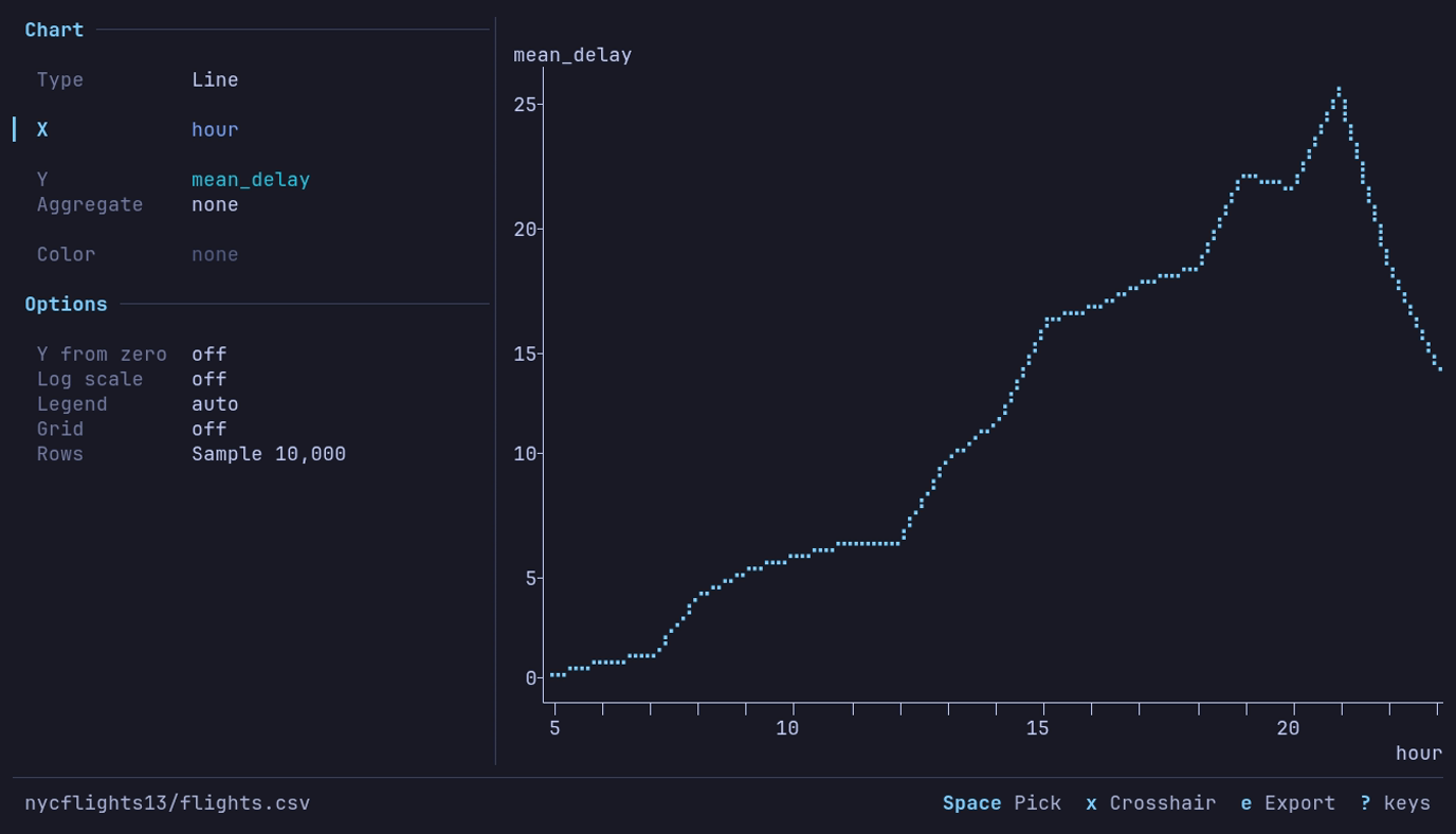
When does a JFK departure leave late? In the evening, 26.1 minutes on average
at 21:00. The JFK query, then c
1 on mean_delay, X hour.
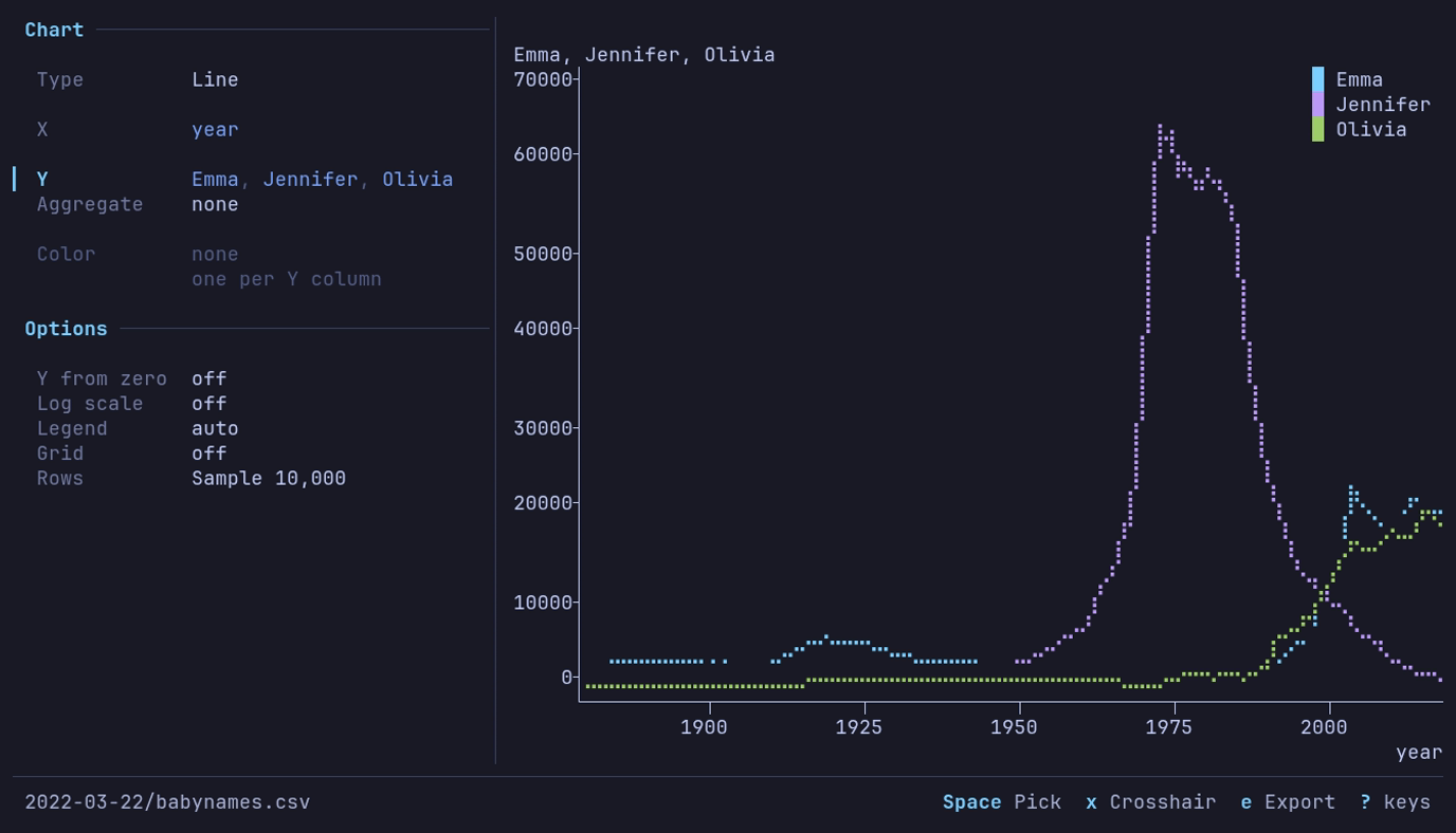
How did three names rise and fall? Jennifer peaks at 63,604 in 1972; Emma and
Olivia rise after 2000. The pivot, then c
1, X year, Y all three.
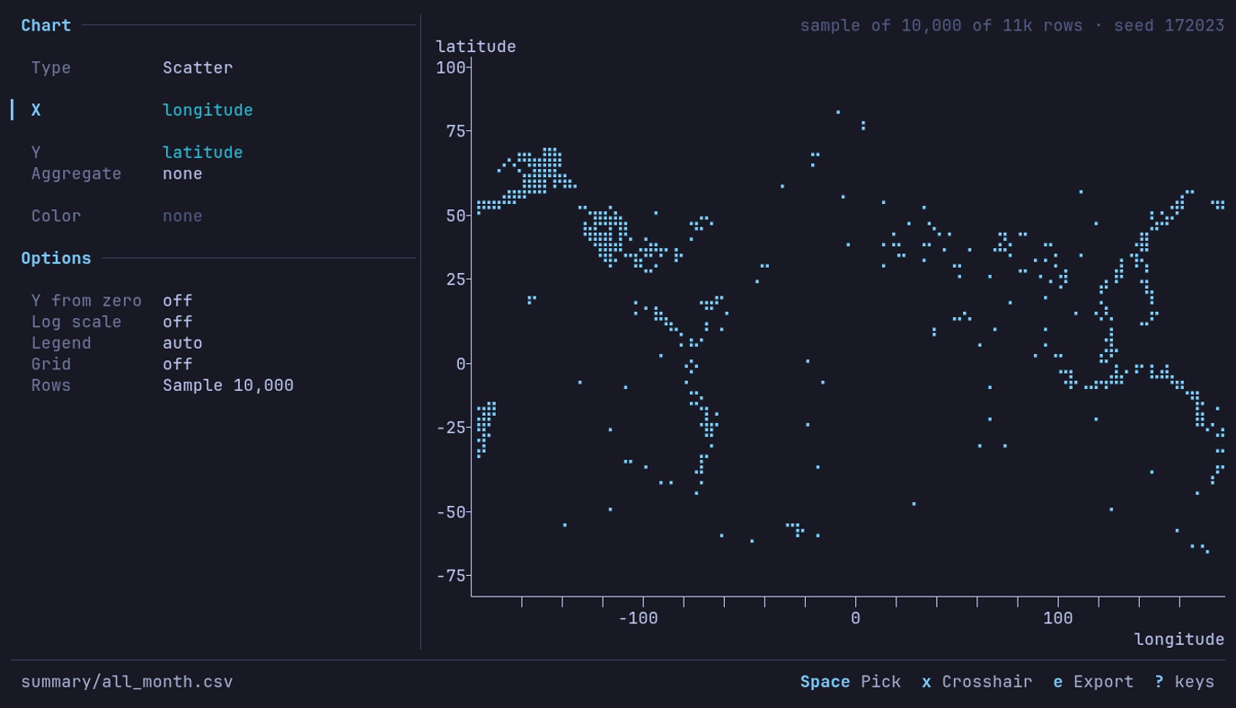
Where does the earth shake? Around the Pacific. c 2 on
latitude, X longitude. The feed rolls, so your month shows its own points.
Large tables
| Option | What it does |
|---|---|
| Rows | Rows a chart without an aggregate reads. A larger table is sampled across all of it, and the chart says so at the right of the title row, with the sample’s seed: sample of 10,000 of 3.5M rows · seed 42891. Every row reads the whole view. A Line over a larger table is not sampled: see below |
| Aggregate | Reads every row, whatever the sample size |
| The view’s sample | Read whole: the Rows row is hidden, and the title row names the sample and its seed: sample 100,000 of 3.48M · seed 42891 |
On Rows:
| Key | Does |
|---|---|
| ← → or Space | Switch between Sample 10,000 and Every row (36.8M), which names the view’s rows once the table has counted them |
| Digits | Type a sample size in place: 50000, 50,000, 50k, 250k, 2m. A size of at least the view’s rows is Every row |
| Backspace | Edit the size being typed |
| Enter | Read what the row says. Leaving the row reads it too |
| Esc | Put the row back as it was, without reading |
Nothing is read while you edit the row: the chart stays as drawn, and the
line under the row says Enter to read. An invalid size (12x, 0) says why
there and is not read. Sample keeps its size while Every row is
chosen.
The sample is drawn as the analysis tools
draw theirs, with the same seed: 50 blocks of rows from one Parquet or IPC file, or one
streamed pass over anything else. Changing an option, or charting columns
already read, reuses the same rows without reading the table again. An
exported chart carries the same notes under the plot. The default size comes
from chart_rows in the
[analysis] config section and is 10,000.
A Line chart with no aggregate and no color, over more rows than the sample
size, draws an envelope instead: X is cut into half as many steps as the sample
size, and each step draws its lowest and highest value, so every peak of a
waveform or a long time series stays on the plot where a sample would miss it.
It reads the view in two streamed passes: one for the row count and X’s range,
then one for the steps. The title row says so: min and max of 192M rows in 5,000 steps. Scatter still samples. So does a Line over Parquet read in place
from S3, GCS or Azure, since the envelope would download the whole file twice.
Keys
| Key | Action |
|---|---|
| 1–7 | Switch the type directly, from anywhere: Line, Scatter, Bar, Histogram, Box, KDE, Heatmap ([ ] step) |
| ↓ ↑ or Tab Shift+Tab | Move between the panel’s rows |
| Space Enter | Open a shelf’s picker, or the Color values; toggle an option, or take its next value. The panel applies as it changes, so Enter acts as Space does |
| ← → | Step the type, the time bucket, the aggregate, cumulative, bins, range, order, smoothing window, raw line, trend, over or sample size (+ - too, PgUp PgDn for bigger steps on the sample size); on a shelf of one column or on Color, the previous or next column; flip a toggle |
| g | Grid on or off |
| x | The crosshair, on a line or scatter chart |
| y | Copy a scatter’s trend fit |
| e | Export the chart |
| ? | Help |
| Esc | Back to the table |
In a picker, type part of a name to narrow the list and use ↑ ↓ to move. Enter chooses. Space chooses too until you type, and then it types a space. On a line or scatter chart’s Y on Color and on the Color values, Space toggles an entry in or out instead. Tab or Shift+Tab chooses and moves to the next or previous row, and Esc closes just the picker.
Export
e in the chart view opens the export dialog, with the cursor on its path. Type a
path and press Enter; the keys are those of every
dialog, and Ctrl+P recalls a
path exported to before. A path ending .png, .svg or .pdf takes that
format; any other path gets Format’s extension added (chart.v2 writes
chart.v2.png). You are asked before an
existing file is overwritten, and a failed export leaves it as it was
(Overwriting). A blank path, or a failed
write, keeps the dialog open with the reason under the fields.
| Field | What it sets |
|---|---|
| Format | PNG, SVG or PDF; SVG and PDF are vector, their text set as outlines |
| Style | Light: white, with colors that stay apart for color-blind readers and in print. Dark: the terminal theme’s colors. Transparent: Light with no background |
| Size | A preset, below; typing Width or Height makes it Custom |
| Legend | Line ends names each line at its right end, shortened in the middle if it would run past the page’s margin, the default for line and KDE charts; other charts default to a legend at the top right. Below lists the names in rows under the chart, so long names cost height rather than width; a name wider than the chart is shortened in the middle. Or a corner, or Off. A chart whose legend is off exports with it off |
| Opacity | Scatter: Auto (the default) draws points opaque up to 1,000 and fainter as there are more, down to 15% from 100,000, so a dense cloud shows where it is densest; or 100%, 50%, 20% |
| Point size | Scatter: Small, Medium (the default) or Large, 1.6, 2.4 or 3.6 pt |
| Line width | Line, colored or not: Thin, Normal (the default) or Bold, 1, 1.5 or 2.5 pt; the legend’s swatches follow |
| Y from zero | Line: On includes zero in the Y axis. It starts as the chart’s Y from zero option. Not offered for a log Y. Bars always start at zero |
| Title, Description | Over the chart. The description starts as the plot’s title row, which says how the chart is made: Mean by month, colored by carrier; empty when it has none. The Y column is named over the plot’s left edge, as on screen |
| Notes | Under the chart, after what the chart says about its rows (a sample, values a range left out) |
| Source, Byline | The last line: Source: … and the byline. Source starts from the catalog entry when the dataset came from one: its name, publisher and license |
| Recipe | Include (the default, from chart.export_recipe) writes how the chart was made into the file; Omit writes no datui metadata at all |
| Size | Pixels | Prints at |
|---|---|---|
| Slide 16:9 | 1920 × 1080 | 10 × 5.6 in |
| Document | 1600 × 1000 | 10 × 6.25 in |
| Square | 1200 × 1200 | 8 × 8 in |
| Single column | 1050 × 788 | 3.5 × 2.6 in, 300 dpi |
| Double column | 2100 × 1300 | 7 × 4.3 in, 300 dpi |
| Custom | 16 to 8,192 a side | the last preset’s resolution |
The recipe is a JSON document that reads back as a view:
| Key | Holds |
|---|---|
datui | The version that wrote it |
source | The path, or the URL without its user, password, query string or fragment |
table | The table of a file of tables, when it is one |
rows | What the chart read: the sample with its seed, or every row |
settings | The view’s: the sample’s scope, method, size, seed and how it was drawn, with the view it was drawn through; the query, filters, sort, column layout and types, reshape; the chart, its options and its export settings, the dialog’s words included |
The image is the same either way. The recipe can carry paths, bucket names and query values, so choose Omit before sharing a file that should not show them.
| Format | Recipe in |
|---|---|
| PNG | An iTXt chunk, keyword datui-recipe |
| SVG | A <metadata> element, the root’s first child |
The document info, /DatuiRecipe |
datui -c chart.export_recipe=false
Text is set in IBM Plex Sans, bundled with datui, so a chart comes out the same on every machine; a character it lacks falls back to a system font. Its size follows the page: smaller on a journal column, larger on a slide. A bar chart exports up to its first 100 bars and counts the rest.
Colors
Series take chart_1 through chart_10 from the
theme, in order; bars and histograms take
chart_1, Other dimmed, and the grid chart_grid. The Dark export takes
the same slots, its background background, and its text text_primary and
text_secondary.
Two series never share a color. A slot the theme gives the same color as an
earlier one is skipped. On a 256- or 16-color terminal, or under NO_COLOR,
slots are compared as the terminal shows them, and a chart draws one series per
distinct color. So a 16-color terminal draws fewer series (top 4 of 16 by rows), with Other for the rest when it is on. A Dark export skips a
repeated slot too, and otherwise always has all ten.