Query data
: opens the command line in the footer: a row number, or a query in
SQL or q over the table. The prefix says what Enter will do: row:
while the line is digits alone, else sql: or q:.
Ctrl+T switches between SQL and q, keeping what is typed,
and the line opens in that language next time. With a query in effect the line
opens on its text, in its language, selected: typing replaces it, the arrows
edit it.
| Prefix | What you type | Example, on NYC flights (2013) |
|---|---|---|
row: | A row number | 1200 |
sql: | SQL over the table named df | SELECT carrier, COUNT(*) AS flights FROM df GROUP BY carrier ORDER BY flights DESC |
q: | Datui’s short language, a subset of q, described below | select flights: count flight by carrier |
| Key | Action |
|---|---|
| Enter | Go to the row, or run the query; an empty query returns to the full table |
| Tab | Complete the column name being typed (in SQL, df too) |
| Ctrl+T | SQL or q |
| Esc | Cancel |
| ↑ ↓ | The language’s history |
To keep the rows that hold some text, find it with / and press Ctrl+G.
Running a query, or clearing one, starts a fresh view: sidebar filters, sort,
frozen columns and pivot/melt are dropped. Apply them after the query. A SQL
ORDER BY on columns marks their headers ▲ or ▼, as a sort does, until a
sort from the sidebar replaces it. The
command line stays open until the query’s first rows are in. A query that fails on
the data is not applied: the reason shows under it, the table keeps what it
showed, and the query stays to fix.
To start in q, set query.default_mode:
[query]
default_mode = "q"
A build without the sql feature
has q alone.
Run a query
Open NYC flights (2013) from Example datasets on the home screen: 336,776
departures from JFK, LaGuardia and Newark, delays in minutes. When does a JFK
departure leave late? At sql::
SELECT hour, AVG(dep_delay) AS mean_delay, COUNT(dep_delay) AS flights
FROM df
WHERE origin = 'JFK'
GROUP BY hour
ORDER BY hour
Statements are split over lines here to read; type them on one line, or press Alt+Enter for a new line. 19 rows, one per scheduled hour. The mean delay climbs from 0.5 minutes at 5:00 to 26.1 at 21:00. In q the same query is one line:
select mean_delay: avg dep_delay, flights: count dep_delay by hour where origin = "JFK"
Which airlines arrive late?
SELECT carrier, AVG(arr_delay) AS delay, COUNT(*) AS flights
FROM df
GROUP BY carrier
ORDER BY delay DESC
F9 is last at +21.9 minutes; AS, at −9.9, arrives early on average. Press Enter on AS to see its 714 flights: every one is Newark to Seattle. Esc comes back. See Drill down a GROUP BY.
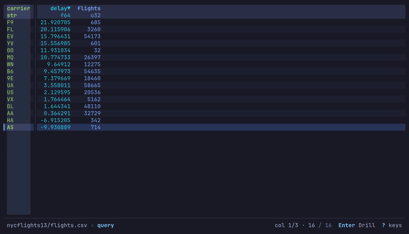
Which airlines arrive late? F9, by 21.9 minutes on average; AS arrives early. :, the query, Enter, then G to AS.
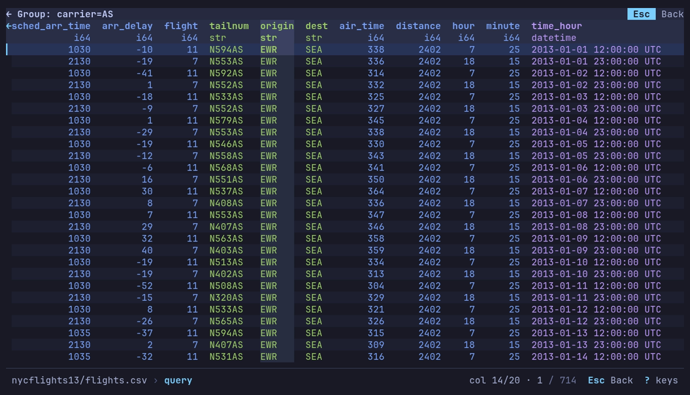
Where does AS fly? Enter on AS: its 714 flights, Newark (EWR) to
Seattle (SEA). Esc goes back.
SQL
SQL mode runs the SQL that the bundled version of
Polars supports,
not the full SQL standard. A statement reads one table, df:
df is | While |
|---|---|
| The group’s rows | Drilled down into a group |
| The pivot or melt result | A pivot or melt is in effect |
| The data as loaded | Otherwise |
Sidebar filters and sort are not part of df, and neither is the previous
statement’s result: each statement starts from df again.
A statement’s rows come back in one order on every read: joins, unions,
DISTINCT and groupings keep the order of the rows they read (a grouping that
drills down, with no ORDER BY or LIMIT, is sorted by
its keys instead), and rows that an ORDER BY ranks equal keep the order they
come in. Paging through the result never repeats a row or skips one, and a
LIMIT without ORDER BY keeps the same rows.
Write SQL
| Key | In SQL |
|---|---|
| Tab | Complete the column name, or df, being typed. Press again for the next match |
| Alt+Enter | Start a new line |
| Enter | Run the statement |
| ↑ ↓ | Move between lines; past the first or last, walk the history |
- The columns of
dfare listed under the input in their types’ colors, narrowed to the name being typed. Names with spaces complete in double quotes:"Team 1"; in q, ascol["Team 1"]. - A long statement wraps onto a second line, then scrolls within the two.
- An empty input shows an example to start from:
SELECT * FROM df WHERE ....
When a statement fails on a value that will not convert, the reason names the column, the values that failed and SQL that gets past them:
| Failure | Try |
|---|---|
STRPTIME meets text that does not match the format | Trim it first: STRPTIME(SUBSTR(Date, 1, 15), '%a %b %d %Y'), or REPLACE |
CAST meets text that is not a number | TRY_CAST(col AS INT), which reads it as null |
CAST(col AS DATE) meets a date not written YYYY-MM-DD | STRPTIME(col, '%d/%m/%Y') with the format it is written in |
The count is exact when the whole column was checked before the run stopped. Otherwise it says “At least N”, from the rows read so far.
Dates and messy text
Premier League (2020-21) writes dates as Sat Sep 12 2020, and twelve
postponed matches as Tue Jan 12 2021(P). Scores are text such as 4–3, with
an en dash. SQL takes both apart:
SELECT Round,
       CAST(STRPTIME(SUBSTR(Date, 1, 15), '%a %b %d %Y') AS DATE) AS match_date,
       "Team 1" AS home, "Team 2" AS away,
       CAST(SPLIT_PART(FT, '–', 1) AS INT) + CAST(SPLIT_PART(FT, '–', 2) AS INT) AS goals
FROM df
ORDER BY goals DESC, match_date, home
SUBSTR drops the (P). Two matches had nine goals: Aston Villa 7–2
Liverpool on 2020-10-04 and Manchester Utd 9–0 Southampton on 2021-02-02.
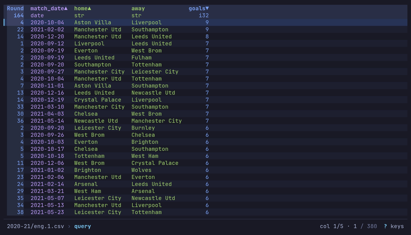
Which matches had the most goals? :, the query, Enter:
match_date is a date and goals a number, two nine-goal matches first.
NYC flights has a time_hour timestamp, but it is in UTC, so a late-evening
departure lands on the next day. The local date is in year, month and day:
SELECT DATE(CONCAT_WS('-', year, month, day)) AS flight_date,
       COUNT(*) AS flights, AVG(dep_delay) AS delay
FROM df
GROUP BY flight_date
ORDER BY flight_date
365 rows, one per day of 2013. Chart flight_date against delay as a line
and 2013-03-08 stands out at 83.5 minutes.
A date or datetime past the calendar’s range, such as a sentinel of
i64::MIN + 1 microseconds, has no calendar text:
| In a query | A date past the calendar |
|---|---|
.str, .format, like, .part, .slice, .replace, .strip, ^ with text | Its stored number, as the table shows it: -9223372036854775807 us since 1970-01-01 UTC |
SQL CAST(... AS VARCHAR), ||, CONCAT, STRFTIME; COALESCE, CASE or UNION with text | Its stored number |
.date, .time, .year, .month_start and the other date parts; SQL date functions and INTERVAL arithmetic | Null |
SQL CAST(... AS TIMESTAMP); ^, COALESCE, CASE, GREATEST or LEAST with a datetime | Null when the datetime cannot count it |
A nanosecond datetime only spans 1677-09-21 to 2262-04-11. Near those ends,
such as pandas’ Timestamp.max:
| In a query | Near the ends of the nanosecond range |
|---|---|
.month_start | Null within a month of 1677-09-21 |
.month_end | Null within a month of either end |
SQL INTERVAL arithmetic | Null when the interval could carry it past an end |
With a time zone: .date, .time, .doy and the rows above | Null within a day of either end |
| A date cast to a nanosecond datetime or met with one, as above | Null before 1677-09-22 or after 2262-04-11 |
Drill down a GROUP BY
Press Enter on a row of a GROUP BY result to see the rows behind
it: the rows of df that passed the WHERE and share the row’s keys, with
every column of df, a key that is a column first. A null key shows the rows
whose key is null.
Esc comes back to the grouped rows, cursor and frozen columns as
they were.
On NYC yellow taxis (January 2025), 3.5 million trips, group by a computed key:
SELECT EXTRACT(HOUR FROM tpep_pickup_datetime) AS pickup_hour,
       COUNT(*) AS trips, AVG(tip_amount) AS avg_tip, AVG(fare_amount) AS avg_fare
FROM df
GROUP BY pickup_hour
ORDER BY pickup_hour
24 rows: 18:00 is the busiest hour with 267,951 trips, 4:00 the quietest with 20,033. Enter on hour 4 shows those 20,033 trips.
| Drills | Does not drill |
|---|---|
SELECT keys, aggregates FROM df [WHERE] GROUP BY keys, then any HAVING, ORDER BY, LIMIT | Joins, subqueries, WITH, UNION |
A key named by its column, its select alias, its position (GROUP BY 1) or the same expression as selected | Window functions (OVER), DISTINCT ON, GROUP BY ALL, UNNEST |
Computed keys: EXTRACT(HOUR FROM ts) AS h | A key that is not selected, or written differently in SELECT |
Where a statement does not drill, Enter
inspects the row instead. Where it drills, the footer
says Enter Drill. A result that drills has the
keys that lead it frozen, as a q by does. Without ORDER BY or LIMIT it comes back sorted by its keys,
since Polars returns groups in no fixed order.
q
q is a subset of the q language, not a complete q or q-sql, and it evaluates right to left. Use it where it is shorter than the SQL:
| Dataset | q | SQL |
|---|---|---|
| Palmer penguins | select mean_mass_g: avg body_mass_g by species | SELECT species, AVG(body_mass_g) AS mean_mass_g FROM df GROUP BY species |
| NYC flights (2013) | select mean_delay: (avg dep_delay).round[1] by hour | SELECT hour, ROUND(AVG(dep_delay), 1) AS mean_delay FROM df GROUP BY hour |
| NYC yellow taxis | select trips: count VendorID by tpep_pickup_datetime.hour | SELECT EXTRACT(HOUR FROM tpep_pickup_datetime) AS hour, COUNT(VendorID) AS trips FROM df GROUP BY hour |
| US baby names | select total: sum n by name where name in ["Emma", "Jennifer", "Olivia"] | SELECT name, SUM(n) AS total FROM df WHERE name IN ('Emma', 'Jennifer', 'Olivia') GROUP BY name |
from df is optional and accepted after the columns and by, as in q and like SQL’s FROM df:
select mean_delay: avg dep_delay by hour from df where origin = "JFK".
Right to left means a * b + c is a * (b + c), and (a + b) * 2 > 100 is
(a + b) * (2 > 100): put the comparison first, 100 < (a + b) * 2.
Query syntax has the grammar, every accessor
and more examples on the built-in datasets.
A by clause without aggregates gives one row per group; with aggregates,
one summary row per group. Press Enter on a group to drill down to
its rows; a row above the table names the group, and Esc comes back.
A group without aggregates shows the columns you selected; an aggregated one shows
every column of the rows behind it, after the query’s where, key columns first.
The cursor, frozen columns and column order come back with Esc.
Save a query
A view saves the active query, in its language, with the filters and sort, to replay on the next file of the same shape.